Academic and Engineering Walkthrough
Deductive logic promises necessity. Real solutions are often weaker:
после релиза выросли ошибки
    → релиз, возможно, причина
новый процесс совпал с ускорением delivery
    → процесс, возможно, помог
положительный тест
    → болезнь стала вероятнее
Such inferences often do not make the conclusion impossible. They make it
stronger than the data allow.
Chapter Rule
Always mention the base rate, selection mechanism, alternative causes, and
strength of inference. “Compatible with,” “increases the probability of,” and “causes” are different
claims.
1. Correlation does not imply causation
Let X and Y vary together. At least the following are possible:
X → Y              X вызывает Y
Y → X              обратная причинность
Z → X и Z → Y      смешивающий фактор
X ← Z → Y          общий источник
X ↔ Y              обратная связь
Selection(X,Y)     отбор создал связь
случайность         связь нестабильна
Example:
Teams with a larger number of on-call engineers have more incidents.
Invalid conclusion:
On-call triggers incidents.
Potential confounder: criticality and system scale simultaneously require
more on-call and create more observable incidents.
2. Post hoc: after — means therefore
A произошло.
Затем произошло B.
∴ A вызвало B.
After the deployment the latency increased. Deployment — a strong candidate, but the sequence
by itself is insufficient:
- load changed;
- dependency degraded;
- configuration updated;
- metric recalculated;
- effect started before deployment.
Repair
Synchronize time series, check the changelog, control group,
mechanism, and rollback.
3. Cum hoc: together — means therefore
Conflating simultaneity with causality:
The more the team writes tests, the more bugs it finds. Hence, tests
create bugs.
More tests increase the observability of existing defects. This
measurement effect.
4. Reverse causality
High-performance teams more often implement practice X; therefore, X made them
high-performance.
Maturity may have allowed X to be implemented. To distinguish, a temporal
order, natural experiment, instrumental variable, or other
identification strategy is needed.
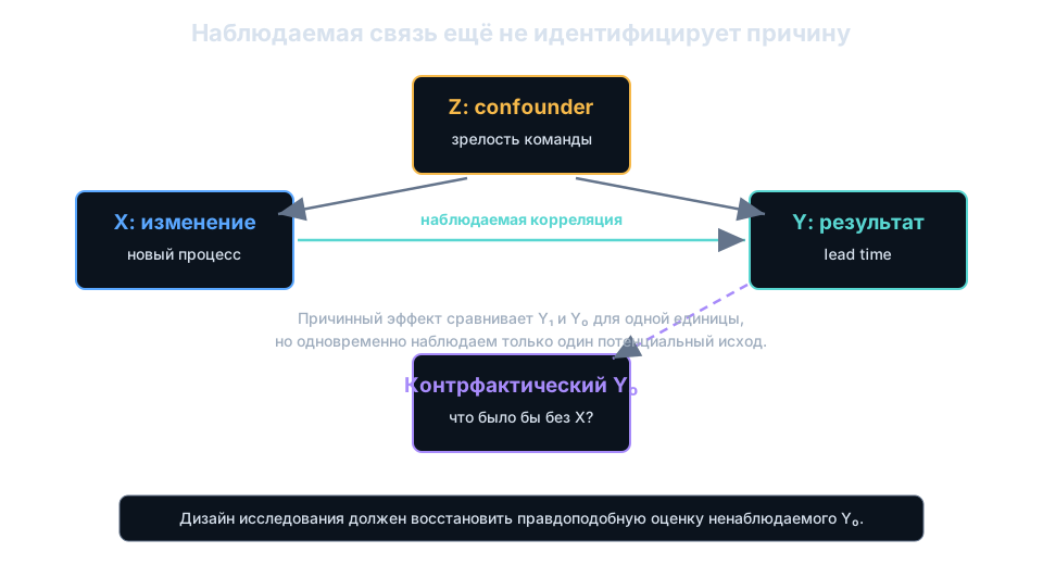
5. Mixing Factor
Z affects both the assumed cause X and the result Y:
Example:
X = использование микросервисов
Y = частота релизов
Z = размер организации, зрелость платформы, автономность команд
Without Z control the correlation does not evaluate the X effect.
Don’t “control everything”
Controlling for a mediator variable or collider can introduce bias.
A causal model is needed before regression.
6. Collider bias
If:
and we select only cases where C, X, and Y can become statistically associated,
although independent in the general population.
Example:
- technical strength of the candidate increases the hiring chance;
- communication strength increases the hiring chance;
- we analyze only those hired.
Among the hired, a false negative correlation may arise: weakness along one
axis is compensated by strength along another.
If the process improves speed through automation, control over the level
of automation will remove part of the real effect of the process. The choice of variables depends
on the question: overall effect or direct?
8. Single Cause Fallacy
A complex result is explained by one factor:
The project failed due to poor architecture.
Product demand, budget, dependencies, team, deadlines, governance are possible.
Architecture may be a necessary part of the explanation, not the only one.
Repair — causal graph and mechanism contribution, not a list of guilty parties.
9. Monotonic Causality
Assume: if a little X is useful, more X is even more useful.
code review полезен → больше reviewers всегда лучше
Real curves have saturation and coordination cost. Look for a response function, not
a binary label.
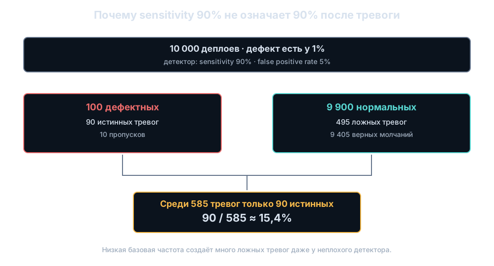
10. Base Frequency
Let:
- 1% of deployments contain a critical defect;
- the detector finds 90% of defective ones;
- it gives 5% false alarms.
After 10 000 deployments:
дефектные:       100 → 90 тревог
нормальные:     9900 → 495 тревог
все тревоги:             585
Probability of defect on alarm:
Not 90%. Test sensitivity is not the probability of the cause after the result.
P(D|+) = P(+|D)P(D) / [P(+|D)P(D) + P(+|¬D)P(¬D)]
The best way to explain is natural frequencies, as above.
11. Prosecutor’s Fallacy
Confuse:
from:
If a profile match occurs once in a million, it does not mean that
the probability of innocence of the specific found person is one in a million.
Needed:
- search population size;
- suspect selection method;
- other evidence;
- measurement errors;
- evidence dependency.
Engineering analogy: a rare fingerprint in the logs can occur for several
reasons, and searching through billions of events almost guarantees random matches.
12. Protection Fallacy
Opposite extreme:
In the city, two people could leave such a trace, meaning the evidence means almost nothing.
You need to update the probability taking into account the entire set of independent and dependent
evidence, rather than discarding a strong likelihood ratio.
13. Conjunction Fallacy
Conjunction cannot be more probable than each part:
But the detailed history seems more plausible:
Сервис упал.
Сервис упал из-за race condition после rollout новой версии.
The second description is more representative, but logically leaner.
When evaluating scenarios, separate the brightness of the story from the probability of the multitude.
14. Gambler’s Fallacy
After a series of results, a “compensation” is expected in an independent process:
Five consecutive builds were green; the next one will definitely fail.
If the trials are independent and the probability is constant, past outcomes do not change the next one.
But the series may be evidence of a changed process: flakiness,
autocorrelation, wear. First, check independence.
15. Hot-hand and clustering illusion
People see runs in random noise or, conversely, consider any run an illusion. The real process may have dependencies. A model of expected run length and a check against it are needed.
16. Law of Small Numbers
A small sample is perceived as a population miniature:
Три кандидата из источника X не прошли.
Значит, источник X плохой.
A small sample has high variance. Show the confidence interval and the
minimal practically significant effect.
17. Hasty Generalization
The conclusion goes beyond the covered population:
Five backend teams accelerated after the practice; therefore, it will accelerate any
team.
Check:
- selection method;
- size and diversity;
- mechanism portability;
- excluded cases;
- observation period.
18. Non-representative sample
Convenience sample
We surveyed those who are easy to find.
Self-selection
Those who are particularly satisfied or dissatisfied respond.
Non-response
Systematically non-responding individuals differ.
Coverage bias
A part of the population could not get into the sample.
Healthy worker / survivor selection
We observe only those who have survived the process.
19. Survivorship Bias
They study successful projects and derive their practices as reasons for success, not seeing
failures with the same practices.
Все заметные стартапы нарушали правило X.
The archive may contain thousands of unnoticed startups that violated X and shut down.
Repair:
requires both successful and unsuccessful cases.
20. Regression to the Mean
After an extreme result, the next one is usually closer to the average even without
intervention.
Команда провалила худший спринт.
Провели жёсткую встречу.
Следующий спринт лучше.
∴ жёсткая встреча помогла.
Possibly, the first sprint was a random extremum.
Use control, multiple periods, and a trend model.
21. Selection Bias
Objects are selected due to high/low results, then the change is measured.
Regression is almost inevitable.
Example: optimize only the slowest queries based on a noisy one-day
measurement; part of the “speedup” will happen without changes.
22. Multiple comparisons
At a significance level of 0.05, out of 100 independent null tests on average about
five will give p < 0,05.
If check:
- 20 metrics;
- 5 segments;
- 4 windows;
but shows the best result, the nominal p-value loses its meaning.
Solutions:
- preregistration;
- adjustment of multiple checks;
- separation of exploratory and confirmatory analysis;
- independent replication.
23. P-hacking
Research flexibility is used until the desired result is achieved:
- change the sample;
- remove outliers after viewing;
- stop the collection at
p < 0,05;
- choose a metric and model post hoc;
- try transformations without accounting for multiple attempts.
The problem is not in one p-value, but in the hidden solution space.
24. Optional stopping
Continuously checking the test and stopping at success means changing
the distribution of statistics.
Use:
- fixed horizon;
- sequential tests with a valid procedure;
- always-valid p-values or a Bayesian design;
- pre-specified stopping rule.
25. Texas sharpshooter
First see a random cluster, then draw a target around it:
In this segment, this week and on this platform the effect is especially strong.
A hypothesis created from data should be checked on new data.
26. Overfitting as a reasoning fallacy
The model explains the noise in the training sample and presents it as a pattern.
Logical analogy: the theory accumulates exceptions until it explains every
old case, but does not make risky new predictions.
Check:
- holdout;
- cross-validation;
- temporal split;
- external validity;
- simplicity relative to data.
27. Simpson’s Paradox
The trend in each group may change or disappear after merging due to
different weights.
Example:
Команда A и B по отдельности ускорились.
Общий средний lead time вырос.
Perhaps the share of complex tasks has moved into one group. Always check:
- component;
- relevant strata;
- causal role of variable stratification.
Automatic preference for an aggregate or groups is not possible; the choice poses a causal
question.
28. Denominator Fallacy
Ошибок стало на 50% больше.
Without the number of requests, it is unknown whether the error rate increased.
errors / requests
affected users / active users
incidents / deploys
Display the numerator, denominator, and absolute numbers.
29. Relative and Absolute Risk
The risk increased from 1 in a million to 2 in a million:
- relative growth: 100%;
- absolute growth: 1 per million.
Both digits are correct and answer different questions. Manipulation — showing only
the convenient one.
30. Average without Distribution
Average latency 100 ms may hide:
- 99% at 10 ms and 1% at 9 seconds;
- all users around 100 ms;
- two different segments.
Need:
- median and quantiles;
- distribution;
- segments;
- tails;
- temporal dynamics.
31. Ecological and Atomic Errors
Environmental
A group property is transferred to an individual:
In teams with high seniority, the speed is higher; thus, any senior is faster
than any junior.
Atomic
Move individual links to groups:
A more experienced engineer is usually faster; therefore, increasing the average experience
of the team always increases throughput.
At the team level, coordination, specialization, and task distribution are in effect.
32. Precision Error
Вероятность проекта — 73,42%.
Two decimal places do not create knowledge. Show:
- range;
- sensitivity to preconditions;
- model calibration;
- source of uncertainty.
33. Causal Protocol
- Define X, Y, and the measurement moment.
- Formulate the counterfactual question: what would happen to Y without X?
- Draw the assumed DAG.
- Find confounders, mediators, colliders.
- Describe the mechanism.
- Define the intervention or identification strategy.
- Fix the sample and missingness.
- Specify the primary outcome and horizon.
- Show the absolute effect and uncertainty.
- Check robustness and transportability.
flowchart LR
X["Изменение X"] --> M["Механизм M"]
M --> Y["Результат Y"]
Z["Контекст Z"] --> X
Z --> Y
S["Отбор S"] --> X
S --> Y
C["Контрольная группа /<br/>контрфактическая оценка"] -. сравнение .-> Y
34. Walkthrough: “After AI implementation, the speed increased by 30%”
Clarifications:
Что такое скорость?
Какая единица анализа?
Кто попал в выборку?
Как выбран период до/после?
Изменилась сложность задач?
Были параллельные изменения?
Есть контроль?
Как учтено качество и rework?
Кто не использовал инструмент?
Это intention-to-treat или usage effect?
A correct bounded derivation may sound like:
The median time to complete a selected task class by pilot participants
decreased by 30% compared to their previous period. The before/after design
does not isolate the tool from training, task changes, and participant selection;
the result justifies a controlled next experiment, but not a general causal claim.
35. Checklist
- Are conditional probabilities not swapped?
- Is the base rate specified?
- Are numerator and denominator present?
- Is the relative effect supplemented by the absolute one?
- Does the sample cover the target population?
- Are we seeing only survivors?
- Is the extremum not regressing to the mean?
- Were the hypothesis and metric chosen before viewing?
- Are multiple checks and stopping rule considered?
- Is the aggregate checked across relevant groups?
- Is correlation supplemented by a causal graph?
- Is a confounder not confused with a mediator or collider?
- Is an alternative explanation checked?
- Are uncertainty and generalizability indicated?
36. Tasks
- The detector has sensitivity 95%, false positive rate 2%, base defect rate
0.1%. Calculate
P(дефект | тревога) using natural frequencies.
- After mandatory training, the number of registered incidents increased.
Provide three causal models.
- Only projects surviving three years were studied, and a common practice was
found. What denominator is missing?
- The team selected the worst 10 endpoints and after optimization saw
improvement. Where could regression to the mean occur?
- The experiment showed a 20% increase in conversion for mobile and desktop, but
overall conversion decreased. Construct a possible Simpson’s example.
- Out of 200 metrics, three significant ones were found. What data is needed for
interpretation?
Sources
What’s next
Statistical error describes the structure of data and output. Cognitive
bias describes why attention and evaluation systematically push us toward
certain errors. These levels are connected, but not identical.
Cognitive biases